
DDL + INSERT for TABLES used in questions
PRODUCTS
CREATE TABLE IF NOT EXISTS products (
   product_id SERIAL,
   product_name varchar(500),
   product_category varchar(250),
   random_desc text
);

INSERT INTO products (product_name, product_category, random_desc)
     SELECT 'Product '||floor(random() * 10 + 1)::int
          , 'Category '||floor(random() * 10 + 1)::int
          , left(md5(i::text), 15)
       FROM generate_series(1, 1000) s(i);
SALES
CREATE TABLE IF NOT EXISTS sales (
   id SERIAL,
   sales_date TIMESTAMP,
   sales_amount NUMERIC(38,2),
   sales_qty INTEGER,
   discount NUMERIC(38,2),
   product_id INTEGER
);

INSERT INTO sales (sales_date, sales_amount, sales_qty, product_id)
     SELECT NOW() + (random() * (interval '90 days')) + '30 days'
          , random() * 10 + 1
          , floor(random() * 10 + 1)::int
          , floor(random() * 100)::int
       FROM generate_series(1, 10000) s(i);
CONTACTS
CREATE TABLE IF NOT EXISTS contacts(
    imie_nazwisko TEXT,
    gender TEXT,
    city TEXT,
    country TEXT,
    id_company INTEGER,
    company TEXT,
    added_by TEXT,
    verified_by TEXT
);
INSERT INTO contacts VALUES
    ('Krzysztof, Bury', 'M', 'Kraków', 'Polska', 1, 'ACME', 'Person A', 'Person B')
  , ('Magda, Kowalska', 'F', 'New York', 'USA', 2, 'CDE', 'Person C', 'Person A');
NOTICE: This table has some structural errors (ex. normalization) on purpose ... check questions.
You can use SQL Fiddle in browser for online execution - HERE
Click on Question to find the answer.
What does SQL stand for? What are the elements of a database query language? #basics #theory
SQL (Structure Query Language) is a database query language.
SQL can be divided into several parts:
- DDL - Data Definition Language - part of the SQL language, responsible for creating, modifying or deleting database objects, operations such as CREATE, ALTER, DROP.
- DML - Data Manipluation Langugage - a set of SQL statements that allows you to perform INSERT, UPDATE, DELETE operations (adding, updating, deleting rows).
- DQL - Data Query Language - the basis of data retrieval, i.e. SELECT.
- DCL - Data Control Language - an element that allows you to add or remove permissions, GRANT / REVOKE.
- DTL / TCL - Data Transaction Language / Transaction Control Language - the part responsible for handling transactions: COMMIT, ROLLBACK, SAVEPOINT.
What is a database management system (DBMS)? #basics #theory
DBMS - Database Management System - is a set of rules (system) described by computer programs that allow the manipulation (manage) of the attribute values of several different types of entities arranged in a sensible way (database).
What is DDL in the context of SQL? #basics #theory
DDL - Data Definition Language, is an element of the database query language, which aims to create, modify and delete elements of the database structure - tables, schemas, indexes, etc.
The key elements of the syntax include the operations: CREATE, ALTER and DELETE.
Although the above operations are part of the standard, their additional elements are implemented differently by different database solution providers. Below are sample definitions of the CREATE TABLE statement from various vendors
CREATE TABLE:
Provide one example of syntax usage for each DDL element. #basics #theory
CREATE: CREATE TABLE sales ( id SERIAL );

ALTER: ALTER TABLE sales ADD COLUMN sales_amount NUMERIC(10,2);

DROP: DROP TABLE sales;
What is DCL in the context of SQL. #basics #theory
DCL (Data Control Language) is an element of the database query language that aims to grant and revoke access to database objects.
The key elements of the syntax include the following operations: GRANT / REVOKE (DENY)
- GRANT - grant access to database objects
- REVOKE (DENY) - denies access to database objects
What is TCL in the context of SQL. #basics #theory
TCL (Transaction Control Language) - is an element of the database query language, which aims to manage transactions in the database.
The key elements of the syntax include the following operations: COMMIT, ROLLBACK, SAVEPOINT.
- COMMIT - confirms the transaction and all actions performed in it.
- ROLLBACK - rolls back a transaction and all actions performed in it that affect the structure of the database and the data itself.
- SAVEPOINT - saves state that can be referenced inside a transaction.
What elements of the database structure can we distinguish (elements as database layers, e.g. tables, indexes, etc.)? #basics #theory
Typical elements of the database structure include:
- database schema
- tabels
- columns (attributes/fields)
- poems (records)
- keys/constraints
- views
- indexes
- procedures/functions
What are the standard data types you know - general types plus a rough breakdown of them - based on the database you have the most experience with. #basics #theory
Data types can be divided into:
- alphanumeric
- numerical
- date and time
- boolean
- arrays
- binary
- json/bson
- xml
What are the typical constraints of table attributes (columns)? #basics #theory
- PRIMARY KEY - the primary key of the table (relation) - if it is simple, i.e. one-element, it is an attribute limitation. In the case of a composite primary key, it will be the constraint of the relationship.
- NOT NULL / NULL - the value cannot / cannot be undefined
- UNIQUE - the value must be unique in the entire relationship
- SERIAL / AUTO_INCREMENT - the attribute is of numeric type with automatic increase of the value in the field when the INSERT operation is performed
- DEFAULT value - default value for the attribute
- CHECK condition - limitation of the attribute domain, e.g. AGE column with CHECK restriction > 14, i.e. the value of the AGE attribute must be higher than 14 at the time of performing the INSERT operation
What is a database transaction? #basics #theory
It is nothing more than a method used by the application to group, read and write operations into one logical unit. The result of a transaction is one of two states: Success (the transaction is committed) or Failure (the transaction is canceled or rolled back).
Let's look at a classic transaction example: a bank transaction exchanging funds between two accounts, Account A and Account B. The owner of Account A wants to transfer PLN 100 to Account B. Generally, we have two approaches in this example.
Approach 1:
Operation 1: Account A balance = Account A balance - PLN 100;
Operation 2: Account B balance = Account B balance + PLN 100;
Approach 2:
Operation 1: Account B balance = Account B balance + PLN 100;
Operation 2: Account A balance = Account A balance - PLN 100;
In reality, the whole operation is a bit more complicated (there are checks, business and legal rules of the bank, etc.), but the idea is the same. If a failure occurs while an operation is being performed, we have a problem. Either PLN 100 will evaporate from Account A and will not appear in Account B, or it will appear in Account B, but the balance of Account A will not be changed. A transaction comes to the rescue, as it covers the execution of an operation in one of the Approaches and guarantees: successful execution of both operations (COMMIT), or no changes in the states of both Accounts (rollback / ROLLBACK)
BEGIN [TRANSACTION]
    AccountStateA = AccountStateA - 100;
    AccountBan = AccountB + 100;
END [TRANSACTION] (COMMIT)
What is ACID in relational databases? #basics #theory
A.C.I.D. guarantees security in relational databases.
It is a set of mechanisms that are intended to provide some resistance to errors and problems of relational databases.
A.C.I.D. is an acronym for 4 such guarantors:
- A (Atomicity) - atomicity
- C (Consistency) - consistency
- I (Isolation) - insulation
- D (Durability) - durability
What is concurrency control in databases? What problems do you know about concurrency control? #basics #theory
Concurrency Control - a set of functions provided by a database to allow multiple users to access data simultaneously and perform operations on nothing.
Concurrency Control Problems:
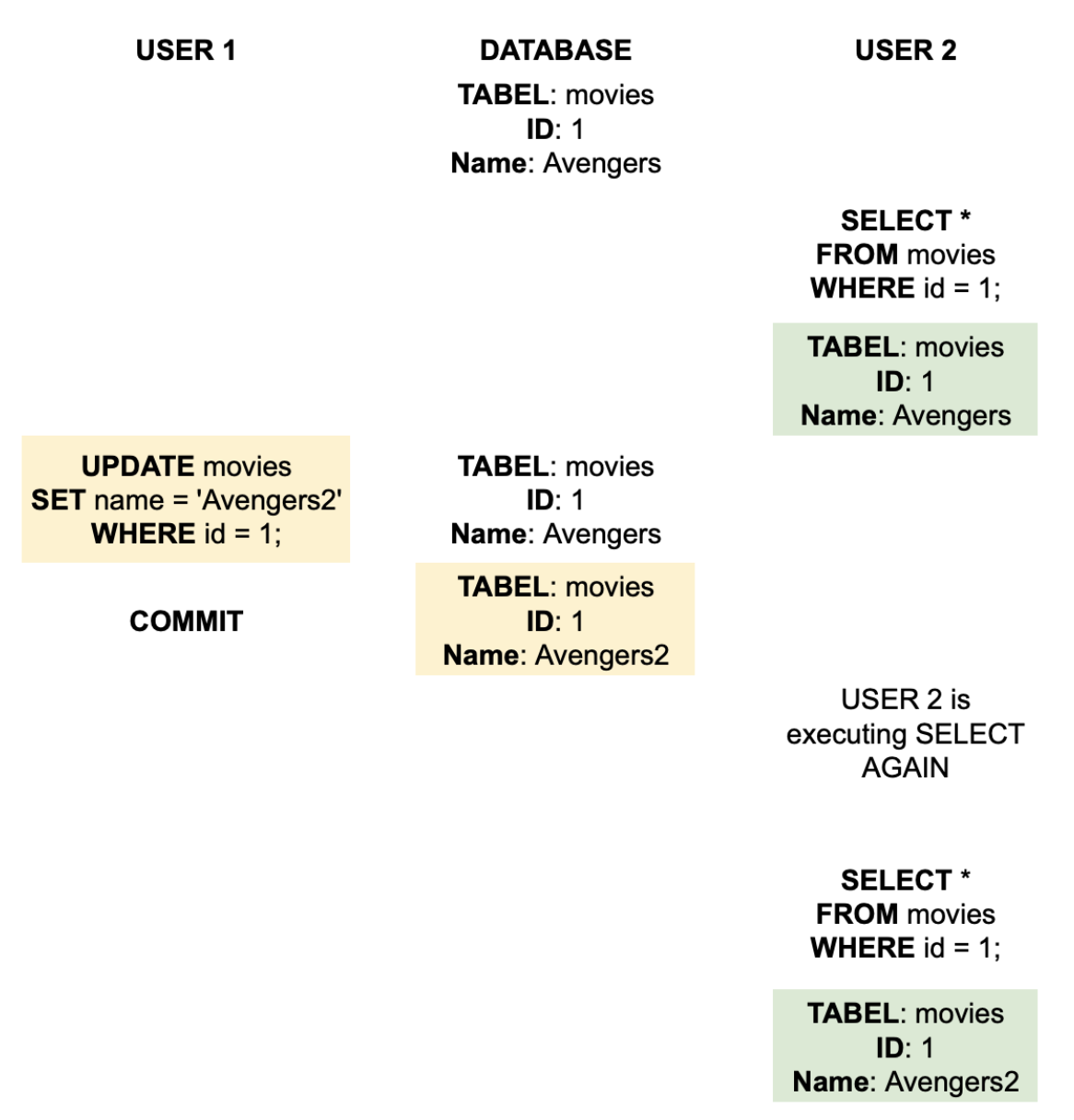
- Dirty Read - reading "updated" (UPDATE) data before it is accepted (COMMIT) by another transaction.
- Phantom Read - the appearance of new records / or the disappearance of existing ones while the same query will be run after executing 1 equivalent query.
- Non-Repeatable Read - causes records from the previous query to appear in their changed form when the query is re-executed.
- Lost Update - causes a pending transaction to be overwritten with another transaction previously initiated by another transaction.
What is a lock in a database? #basics #theory
LOCK occurs when two transactions are waiting for each other to release resources and at least one of them cannot continue its operation.
T1: UPDATE products SET product_name = 'Product 999' where product_name = 'Product 1';
T2: UPDATE products SET product_name = 'Product 998' where product_name = 'Product 2';
T1: UPDATE products SET product_name = 'Product 001' where product_name = 'Product 1';
T2: UPDATE products SET product_name = 'Product 991' where product_name = 'Product 2';
Same rows 'Product1' and 'Product2' are modified from different transactions with COMMIT.
What is isolation in relational databases? #basics #theory
Isolation means that simultaneously executed transactions are isolated from each other - they cannot influence each other. This is especially important in the case of access to the same resource (same table), in the case of access to different objects, the conflict will not occur.
Another definition is one in which isolation is a guarantee in which the parallel execution of a transaction will leave the database in a state as if the operations had been performed in a sequential manner.
It is worth remembering that isolation is an exchange of database integrity at the expense of performance.
Example:
What are transaction isolation levels and what do you know? #basics #theory
Transaction isolation levels are standards/approaches for dealing with transaction concurrency issues.
- Read Uncommited - the least restrictive, allows 3 types of reads (Dirty, Phantom and Non-Repeatable Reads). Probably not used in commercial databases.
- Read Commited - allows the query to access data that has been accepted (COMMIT). No Dirty Reads, allow Phantom and Non-Repeatable Reads. The most commonly used insulation level.
- Repeatable Read - guarantees the consistency of readings. Only allows Phantom Read.
- Serializable - the most restrictive isolation level (does not allow Dirty, Non-Repeatable and Phantom Reads). Each transaction is treated as if it were the only transaction taking place in the database at that time.
What is the difference between Read Committed and Serializable isolation levels? #basics #theory
- Read Committed - good separation between consistency and concurrency. Good for standard OLTP (OnLine Transaction Processing) applications in which there are many concurrent, short-lived transactions, rarely of which conflicts. Better performance.
- Serializable - good for databases with many consistent transactions. Lower performance due to higher blocking. Mainly used in databases with read-only transactions that run for a long time (analytical queries, see OLAP - OnLine Analytical Processing).
What is database normalization? #basics #theory
Database normalization is a technique for organizing data in a database, it is a systematic methodical approach of "breaking up" tables to eliminate repetitions and unwanted features of adding, deleting and updating rows.
Two key goals of standardization:
- Representing facts about the real world in an understandable way;
- Reducing redundant fact storage and preventing incorrect or inconsistent data;
INSERT - problems with lack of normalization
The city (CITY) column in the CONTACTS table is a good example to consider non-normalization problems in the context of an INSERT operation.
When adding 100 contacts from Poznań, we assign the same text information to all records. On the other hand, if a contact did not provide information about the city (it is not required), we will have to enter the undefined value NULL in this field.
UPDATE - problems with lack of normalization
The COMPANY column in the CONTACTS table is a good example to consider the problems of lack of normalization in the context of the UPDATE operation.
If many contacts work for the same company - ACME - and this company changes its name or disappears from the market. All records will have to have an updated value, omitting a contact and leaving it with the ACME value will result in data inconsistency.
DELETE - problems with lack of normalization
Let's assume that the CONTACTS table is the only place where we store information about the city (CITY). If for some reason we delete all contacts from Poznań, we will not be able to refer to this value for other queries.
What normal forms do you know, list them with a short description? #basics #theory
- 1 Normal Form (1NF) - The table must be a relation and cannot contain any repeating groups.
- 2 Normal Form (2NF) - the table is in 1st normal form, and has exactly one candidate key (candidate key, which is the same primary key) and it is not a composite key (it consists of 1 column).
- 3 Normal Form (3NF) - in 3rd normal form, all non-key attributes must depend on the key of a given table.
- 3.5 / BCNF Boyce-Codd Normal Form (BCNF) - in Boyce-Codd normal form, all attributes, including those belonging to the key, must depend on the key of a given table.
- 4 Normal Form (4NF) - Any table that is intended to represent many many-to-many relationships violates the rules of fourth normal form.
- 5 Normal Form (5NF) - Any table that meets the Boyce-Codd Normal Form criteria and does not contain a composite primary key is in 5th Normal Form.
- 5.5 Domain-Key Normal Form (DKNF) - each table constraint must be a logical consequence of the table domain constraints and key constraints.
- 6 Normal Form (6NF) - a table is in 6th normal form if, in addition to the attribute that is also the primary key, it has a maximum of 1 additional attribute.
What could normalization of the CONTACTS table look like? #basics #theory
1NF - we separate the NAME_SURNAME field.

| NAME| SURNAME | GENDER | CITY | COUNTRY | ID_COMPANY | COMPANY | ADDED_BY | VERIFIED_BY |
|---|---|---|---|---|---|---|---|---|
| Krzysztof | Bury | M | Krakow | Poland | 1 | ACME | PersonA | PersonB |
| Magda| Kowalski | F | New York | USA | 2 | CDE | PersonC | OsobaA |

2NF - we extract the GENDER table based on the GENDER column from CONTACTS.

CONTACTS
| NAME| SURNAME | CITY | COUNTRY | ID_COMPANY | COMPANY | COMPANY | ADDED_BY | VERIFIED_BY |
|---|---|---|---|---|---|---|---|
| Krzysztof | Bury | Krakow | Poland | 1 | ACME | PersonA | PersonB |
| Magda| Kowalski | New York | USA | 2 | CDE | PersonC | PersonA |

GENDER
| NAME| GENDER |
|---|---|
| Krzysztof | M |
| Magda | F |

3NF - we separate the COMPANY table based on the ID_COMPANY and COMPANY columns from CONTACTS.

CONTACTS
| NAME| SURNAME | CITY | COUNTRY | ID_COMPANY | ADDED_BY | VERIFIED_BY |
|---|---|---|---|---|---|---|
| Krzysztof | Bury | Krakow | Poland | 1 | PersonA | PersonB |
| Magda| Kowalski | New York | USA | 2 | PersonC | PersonA |

GENDER
| NAME| GENDER|
|---|---|
| Krzysztof | M |
| Magda | F |

COMPANY
| ID_COMPANY | COMPANY |
|---|---|
| 1 | ACME |
| 2 | CDE |

BCNF - we create a new table CITY_COUNTRY based on the CITY and COUNTRY columns from CONTACTS.

CONTACTS
| NAME| SURNAME | CITY | ID_COMPANY | ADDED_BY | VERIFIED_BY |
|---|---|---|---|---|---|---|
| Krzysztof | Bury | Krakow | 1 | PersonA | PersonB |
| Magda| Kowalski | New York | 2 | PersonC | PersonA |

GENDER
| NAME| GENDER |
|---|---|
| Krzysztof | M |
| Magda | F |

COMPANY
| ID_COMPANY | COMPANY |
|---|---|
| 1 | ACME |
| 2 | CDE |

CITY_COUNTRY
| CITY | COUNTRY |
|---|---|
| Krakow | Poland |
| New York | USA |

4NF - we create a new table CONTACTS_VERIFIED_BY and CONTACTS_ADDED_BY based on the VERIFIED_BY and ADDED_BY columns from the CONTACTS.

CONTACTS
| NAME| SURNAME | CITY | ID_COMPANY |
|---|---|---|---|
| Krzysztof | Bury | Krakow | 1 |
| Magda | Kowalski | New York | 2 |

GENDER
| NAME| GENDER |
|---|---|
| Krzysztof | M |
| Magda | F |

COMPANY
| ID_COMPANY | COMPANY |
|---|---|
| 1 | ACME |
| 2 | CDE |

CITY_COUNTRY
| CITY | COUNTRY |
|---|---|
| Krakow | Poland |
| New York | USA |

CONTACTS_VERIFIED_BY
| CONTACT_NAME | VERIFIED_BY |
|---|---|
| Krzysztof | PersonB |
| Magda | PersonA |

CONTACTS_ADDED_BY
| CONTACT_NAME | ADDED_BY |
|---|---|
| Krzysztof | PersonA |
| Magda | PersonC |
What is a view in SQL? #basics #theory
A view is a persistent definition of a derived table (the result of a SELECT query) that is stored in the database.
In SQL, a table created with a CREATE TABLE query is called a base table. We formally call the result of each SELECT query a derived table. The tables used to define the view are called underlying tables.
Syntax:
CREATE OR REPLACE VIEW view_name AS SELECT ...
DROP VIEW view_name;
View properties:
- does not store data - the view definition is saved in the database. The view itself is only a data reading interface;
- always shows current data - the database always recreates current data from the source tables used to build the view;
Views are used for:
- creating an additional level of table security by limiting access to specific columns or rows of the base table;
- hiding data complexity - when the view definition is a complex SELECT query, the view query itself is visible as a simple query;
- showing data from a different perspective - for example, the view can be used to change the name of a column without changing the actual data stored in the table;
What is the difference between a view and a materialized view (VIEW vs MATERIALIZED VIEW)? #basics #theory
A materialized view, unlike a view, is a SELECT query definition which, when created (and with a specified frequency), saves the query results to a database object, a table.
Data from the materialized view definition are refreshed according to a set schedule (set in the materialized view definition).
As a rule, in the case of complex queries, when a regular view is queried, the entire complex query must be executed. In the case of a materialized view, data is immediately available with an update equal to the last refresh of the view according to the schedule.
What are OLTP transaction systems? #basics #theory
OLTP - OnLine Transaction Processing - is a system focused on short-term, fast transactions.
- data source: operational data; OLTP systems are the original source of data;
- purpose of data: support and control of basic business processes;
- what's in the data: current state of business processes;
- Insert/Update operations: short and fast Insert/Update operations initiated by end users;
- queries: relatively simple and standard queries usually returning a few records;
- processing time: usually very fast;
- needed space: data may take up relatively little space if historical data is archived;
- database structure: highly standardized with a large number of tables;
- data copy and recovery: mandatory data copying; operational data is critical to running a business, data loss usually results in large financial losses and legal liability;
Typical examples are basically most of the enterprise's production support systems - ERP/CRM systems (except analytical modules).
Other Examples: a banking system that supports reading and modifying customer account balances; financial and accounting systems.
What are OLAP analytical systems? #basics #theory
OLAP - OnLine Analytical Processing - are systems focused on providing an analytical model, i.e. preparing data and optimizing the model so that analytical processes are a priority.
- data source: consolidated data; source data of OLAP systems come from various databases/data sources;
- purpose of data: to assist in planning, problem solving and strategic decision-making;
- what's in the data: a multidimensional look at various types of business activities, current state and history;
- Insert / Update operations: cyclical, long-lasting data refreshment, usually using batch files;
- queries: queries that are often very complex and require aggregation;
- processing time: depends on the amount of processed data;
- space needed: large amount of space needed due to the existence of aggregated and historical data;
- database structure: usually denormalized with a small number of tables; star and/or snowflake schemes used;
- data backup and recovery: in addition to backups, reloading data from source systems may be considered as a data recovery method;
A typical example is data warehouses, or generally systems created and optimized for analytical processes.
OLTP vs OLAP, describe the difference between the systems? #basics #theory
OLTP:
- a large number of simple inquiries (transactions)
- systems optimized for quickly adding, deleting and modifying individual records
- usually identified with traditional relational databases
- a small number of inquiries, often regarding many business elements
- systems optimized for quick reading of analytical information (from aggregated data)
- usually associated with data warehouses, supporting the company's business decisions (Business Intelligence systems) and "very large" amounts of data
- data processing (up to the most up-to-date information) may take minutes or hours - we do not assume that the data is up-to-date
What are and what types of aggregate functions do you know in SQL? #basics #theory
Aggregation functions in SQL are a group of functions that, as the name suggests, are used to obtain the result of an operation for a group of records, according to the selected key(s) of the group.
An example may be the sales value divided into product categories.
The most frequently used aggregation functions:
- SUM() - summing
- AVG() - average
- COUNT() - counting occurrences
- MIN() / MAX() - minimum / maximum
- STDEV() - standard deviation
What are and what types of analytical functions do you know in SQL? #basics #theory
Analytical functions are specific types of SQL functions that provide the result for a given row in the context of rows adjacent (preceding/following) the row. We use this type of function, for example, to "rank" data or calculate states (balance).
Most frequently used analytical functions:
- ROW_NUMBER() OVER()
- DENSE_RANK() / RANK() OVER()
- SUM() OVER()
- LEAD() / LAG() OVER()
What is the difference between WHERE and HAVING syntax? #basics #theory
When not used in the context of GROUP BY, they are essentially equivalent.
However, their real use is when data is grouped.
- The WHERE condition filters records from the result before grouping is performed.
- The HAVING condition filters records from the result after grouping has been performed
What do the DELETE and TRUNCATE commands do? What are the differences between them? #basics #theory
Both commands are used to remove rows from a table, but there are some subtle differences between them.
DELETE is a DML (Data Manipulation Language) operation that works at the table row level. With its help, we can delete all rows or one specific row (adding WHERE).
DELETE FROM TABLE_NAME WHERE …TRUNCATE TABLE TABLE_NAME …Transactional
- DELETE, like INSERT or UPDATE, can be accepted (COMMIT) or rolled back (ROLLBACK).
- TRUNCATE in some database systems has the so-called "implicit COMMIT". This means that the COMMIT operation is performed before and after the TRUNCATE operation without the need for additional COMMIT execution.
Note: The above is true in the case of e.g. Oracle, in the case of SQL Server or PostgreSQL the TRUNCATE operation can be rolled back (ROLLBACK).
Reclaiming Place
- DELETE does not reclaim space after deleting rows. Additional VACUUM surgery is needed.
- TRUNCATE reclaims space after rows are deleted.
- DELETE locks the specific table rows that are deleted.
- TRUNCATE locks the entire table.
- DELETE performs AFTER/BEFORE DELETE trigger operations.
- TRUNCATE does not execute triggers.
However, these are quite specific issues, if you want to delve deeper into the topic, I would refer to the specific documentation of the systems you work on.
What is the purpose of the CASCADE option during the DELETE operation in SQL? #basics #theory
When a foreign key relationship is defined between the tables and there are records associated with this relationship, it will not be possible to perform a DELETE operation on the data of the table to which the relationship is created.
The database will inform us that there are records in the relationship between table A and B that we want to delete. To perform this operation, we must first delete the records related to table B or use the CASCADE option.
The CASCADE option removes all rows from table A and all related rows from table B that have a foreign key relationship between the tables.
What is the purpose of the CASCADE option during the DROP operation in SQL? #basics #theory
When there is a relationship between database objects, i.e. object B depends on object A, e.g. view B on table A, performing a DROP operation on object A will not be possible.
The database will inform us that there is a connection in the relationship between object A and B. If we want to delete object A, we must first delete object B or use the CASCADE option.
The CASCADE option removes the object defined for deletion and all objects that use / are created from object A.
What is the IN operator in SQL and what is it used for? #basics #theory
IN is a logical operator used in the WHERE part of the query. It allows you to check whether a value from a given column/function exists/equals any value from the list.
Comparing values against a list is very convenient, an example would be to use such a list on the presentation layer (web page) and then send a request to the database to display only those results for which the user has selected.
The IN operator is basically equivalent to writing multiple OR conditions for the same column and different values. Therefore, it is worth using it in such a case, if only for the sake of readability.
One of the questions that should come to your mind is: "how many values can I use in IN?".
The answer is not clear and will depend on the database.
In SQL Server "a lot" - MORE HERE
For an Oracle database it will be "very little" (1000 according to this article MORE HERE)
Remember that just because we can use multiple values in the IN operator doesn't mean we should. We're just doing a lot of ORing here, and it's not the most efficient approach to querying.
What are the CEIL and FLOOR functions for? Explain the principle of operation of both functions with an example. #basics #theory
The CEIL and FLOOR functions allow you to round a given number to an integer.
You probably remember rounding issues from mathematics. If we have the number 254 and want to round it to the nearest ten, we will get the number 250. If we have, for example, 255, we will get 260.
CEIL (or CEILING) and FLOOR. In the "free" translation: ceiling and floor, and you can already guess what. The CEIL (CEILING) function returns the smallest integer greater than or equal to the value given in the input.
SELECT 8.28 as output_value,
                CEILING(8.28) as positive_value,
                CEILING(-8.28) as negative_value;

Result:
output_value: 8.28
positive_value: 9
negative_value: -8SELECT 8.28 as output_value,
FLOOR(8.28) as positive_value,
FLOOR(-8.28) as negative_value;
Result:
output_value: 8.28
positive_value: 8
negative_value: -9What is the ROUND function? What is the difference in ROUND vs CEIL/FLOOR score. #basics #theory
The ROUND function, like CEIL and FLOOR, allows you to round values. However, rounding is more "mathematical" (i.e. if it is 5 it is up and if it is less than 5 it is down).
Additionally, with this function you can specify to how many decimal places the output value should be rounded.
SELECT 8.49 as output_value,
                FLOOR(8.28) as floor_value,
                CEIL(8.28) as cel_value,
                ROUND(8.49) as rounded_value

output_value: 8.49
floor_value: 8
target_value: 9
rounded_value: 8 (no rounding place after the decimal point was given,
                  default is 0 decimal places)

SELECT 8.51 as output_value,
                FLOOR(8.51) as floor_value,
                CEIL(8.51) as cel_value,
                ROUND(8.51) as rounded_value

output_value: 8.49
floor_value: 8
target_value: 9
rounded_value: 9 (no rounding place after the decimal point was given,
default is 0 decimal places)It depends on the database engine you are using.
For PostgreSQL, the return types for functions are:
- CEIL - same type as input type
- FLOOR - same type as input type
- ROUND - numeric type
What is the ANY operator? Describe the principle of operation with an example. #basics #theory
The ANY operator is used to check whether the searched subset of data (subquery) contains at least one value that meets the used operator.
You can use it in the WHERE section and/or in the HAVING section.
Syntax:
  SELECT column_name
       , ...
    FROM table_name
   WHERE expression / column operator ANY (subquery)
GROUP BY column_name, ...
  HAVING expression operator ANY (subquery)

operator - is one of the available logical operators =, <>, !=, >, >=, <, or <=CREATE TABLE diet_menu (
diet_name text,
diet_ingredients text[]
);
INSERT INTO diet_menu VALUES ('diet1', '{apple, orange, banana}');
INSERT INTO diet_menu VALUES ('diet2', '{apple, banana}');
SELECT *
FROM diet_menu
WHERE 'orange' = ANY (SELECT UNNEST(diet_ingredients));In principle, the actions of the operators are the same. The first SQL standard came into force in 1986, and SQL itself dates back to 1970+, hence the 2 operators, perhaps some backward compatibility?
What is the ALL operator? Describe the principle of operation with an example. #basics #theory
The ALL operator is used to check whether all rows of the searched subset of data (subqueries) meet the used operator. You can use it in the WHERE section and/or in the HAVING section.
Syntax:
  SELECT column_name
       , ...
    FROM table_name
   WHERE expression / column operator ALL (subquery)
GROUP BY column_name, ...
  HAVING expression operator ALL (subquery)

operator - is one of the available logical operators =, <>, !=, >, >=, <, or <=CREATE TABLE diet_menu (
diet_name text,
diet_ingredients text[]
);
INSERT INTO diet_menu VALUES ('diet1', '{apple, orange, banana}');
INSERT INTO diet_menu VALUES ('diet2', '{apple, banana}');
SELECT *
FROM diet_menu
WHERE 'watermelon' <> ALL (SELECT UNNEST(diet_ingredients));In principle, the actions of the operators are the same. The first SQL standard came into force in 1986, and SQL itself dates back to 1970+, hence the 2 operators, perhaps some backward compatibility?
What is the EXISTS operator? Describe the principle of operation with an example. Are the EXISTS and =ANY syntaxes equivalent? #basics #theory
The EXISTS operator is used to search for rows that meet the condition used in the subquery. An enigmatic description, but it comes down to the fact that the result will be the records that exist in the subquery used to build EXIST. The EXISTS operator returns TRUE when the subquery returns 1 or more records.
Syntax:
  SELECT column_name
       , ...
    FROM table_name
   WHERE EXISTS (SELECT column_name
FROM table_name WHERE conditions);JOIN, by its definition, is used to combine tables and display columns from different objects (tables). EXISTS is designed to "filter" the final result based on some subquery.
Example: Display all products (PRODUCTS table) that took part in a sales transaction (SALES table).
SELECT p.*
  FROM products p
 WHERE EXISTS (SELECT 1
                 FROM sales s
WHERE s.product_id = p.product_id);Let's assume we want to display only products for which there is a sales transaction. We can do this with EXIST, but also with ANY.
--EXISTS
SELECT p.*
  FROM products p
 WHERE EXISTS (SELECT 1
                 FROM sales s
                WHERE s.product_id = p.product_id);

-- ANY
SELECT p.*
  FROM products p
WHERE p.product_id = ANY (SELECT s.product_id FROM sales s);The query plan is identical in both cases. If the logical condition is the same, ANY / SOME and EXISTS are interchangeable.
Hash Join (cost=201.25..226.00 rows=100 width=41) (actual time=4.312..4.597 rows=99 loops=1)
Hash Cond: (p.product_id = s.product_id)
    -> Seq Scan on products p (cost=0.00..20.00 rows=1000 width=41) (actual time=0.013..0.138 rows=1000 loops=1)
        -> Hash (cost=200.00..200.00 rows=100 width=4) (actual time=4.278..4.278 rows=100 loops=1)
        Buckets: 1024 Batches: 1 Memory Usage: 12kB
    -> HashAggregate (cost=199.00..200.00 rows=100 width=4) (actual time=4.231..4.240 rows=100 loops=1)
    Group Key: s.product_id
        -> Seq Scan on sales s (cost=0.00..174.00 rows=10000 width=4) (actual time=0.012..2.071 rows=10000 loops=1)
Planning time: 0.431 ms
Execution time: 4.677 ms
How to limit the number of result rows to, for example, 10 elements. Provide examples based on database systems you are familiar with, as well as SQL syntax according to the ISO standard. #basics #theory
You probably know the syntax from the relational database you work with every day:
- LIMIT (including MySQL, PostgreSQL, SQLite, H2)
- TOP (including MS SQL Server)
- ROWNUM (Oracle) - pseudo column in the Oracle database, created when results are generated, specifying the order of retrieved rows
 SELECT * FROM tab LIMIT 10;

 SELECT * FROM tab WHERE ROWNUM <= 10;

SELECT TOP 10 * FROM tab;In a sense, they were forced to do it. This functionality was introduced to the standard for the first time with the SQL:2008 version.
FETCH FIRST n ROWS ONLY allows you to retrieve only n (where n is the number or result of the operation, e.g. (2+2)) rows from the entire result set.
Examples:
SELECT * FROM tab FETCH FIRST 10 ROWS ONLY;What is the equivalent of the IF conditional statement in SQL. Give an example and explain the principle of operation. The solution should be based on a standard, not on an implementation for a given database. #basics #theory
A conditional statement (IF) is a popular structure in programming languages that allows you to check a condition and perform an appropriate action depending on whether the condition is met or not.
Syntax (basic - in programming languages - as pseudocode)
IF <LOGICAL CONDITION>
    THEN <ACTION TO BE PERFORMED WHEN THE CONDITION IS SET>
    ELSE <ACTION TO BE PERFORMED WHEN CONDITION IS NOT MET>
ENDThe construction as above does not exist in standard SQL. However, it exists in Procedural SQL, i.e. in stored procedures and functions executed in the database.
IF exists in SQL and is hidden under the CASE operator
CASE
    WHEN condition1 THEN action1
    WHEN condition2 THEN action2
    ...
    ELSE action_if_others_not_met
END

condition - any operation whose result is a logical value TRUE / FALSE
            (logical operator >, <, =, <> etc.; result from a subquery TRUE / FALSE etc.)

action - an action that is to be performed when a condition is met,
e.g. displaying a column, adding something to a value, etc.If ELSE has not been declared, an undefined value - NULL - will be returned.
You can use the CASE operator in the SELECT syntax itself, in WHERE, in ORDER BY, GROUP BY, etc. However, such an operator always creates additional overhead at the time of execution (for executing the check instruction + performing the action), which will affect performance. In some cases, it is worth considering enumerating columns with the CASE operator earlier (as an element in the pre-use process), adding appropriate indexing and then using the calculated column in SELECT.
Note: In some databases IF exist, e.g. MySQL, or as IIF - Firebird / SQL Server. However, it is not a SQL standard but an overlay on a specific database.
What is the ORDER BY syntax used for? What additional execution options might it contain (NULL/direction handling)? #basics #theory
The ORDER BY operation is used to sort the resulting data.
Do the results have any sorting without ORDER BY.
NO. If the ORDER BY clause is not provided, the query results will be returned in an undefined form. It may be that they appear in the same order as they were added to the source table, but be careful and don't take this for granted.
If you want to get the rows in the desired order, use ORDER BY.
Syntax
  SELECT …
    FROM …
ORDER BY <COLUMN/FUNCTION_NAME> <DESC | ASC> < NULLS FIRST | NULLS LAST >- COLUMN/FUNCTION_NAME - name/names of columns or functions by which sorting is to be performed
- DESC - sort in descending order
- ASC - sort in ascending order
- NULLS FIRST - show undefined values at the beginning of the result set
- NULLS LAST - show undefined values at the end of the result set
Elements used in the ORDER BY syntax do not need to be in the SELECT part.
ORDER BY is one of the last logical elements that will be executed. Therefore, when sorting, we can use aliases - instead of actual column names or field order instead of their names (e.g. ORDER BY 1, 2, 3, where 1, 2, 3 are subsequent columns after the SELECT syntax)
What is a JOIN in SQL database query language? What types of joins do you know? #basics #theory #join
A JOIN is a connection of tables (or table), based on some condition (same columns, logical operators >, < etc.).
In the simplest case, we use joins to map relationships between tables when we want to get a specific result.
Types of joins:
- (INNER) JOIN
- LEFT (OUTER) JOIN
- RIGHT (OUTER) JOIN
- FULL (OUTER) JOIN
What is combining sets using UNION and UNION ALL operations? What is the difference between these operations (UNION vs UNION ALL)? #basics #theory #union #unionall
UNION - is an operation of combining data sets. You can use it to combine records from different tables into one set of records.
What for? Usually when you need to build a list of values from different sets (tables).
Limits
- the number of columns in both queries must be identical
- data types must be compatible in corresponding columns - (in the example above, car_manufacturer cannot be a numeric value and a text value)
- to get sorted results use ORDER BY - you can only use it in the last SELECT. ORDER BY will work on the entire result set. If you want to get sorted results only from the first query, use a subquery for 1 SELECT
- UNION - will combine the results while removing duplicate lines (such as DISTINCT)
- UNION ALL - will combine the results without removing duplicate rows
Attention: In some databases, UNION, in addition to removing duplicates, also sorts the resulting data set (e.g. SQL Server).
What is the difference between INNER JOIN and NATURAL JOIN? #basics #theory #join
INNER JOIN is a type of join in which from two sets (tables or subqueries) we take the values (rows) for which the defined join key is met. This means that the values in the columns from the sets used in the join have the same values (when using “=” columns in a JOIN).
NATURAL JOIN is a type of join in which we take only the common part of two sets (tables or subqueries), but only if there is a column with the same name (or more columns with the same name) in both sets.
What is the difference between LEFT JOIN and RIGHT JOIN? #basics #theory #join
RIGHT OUTER JOIN is a type of join in which from two sets (tables or subqueries) we take all elements from the second set and matching elements (according to the used join key) from the first set. Hence the name RIGHT (referring to the direction of the join) and OUTER referring to the type of outer join (not just the common part).
LEFT OUTER JOIN is a type of join in which from two sets (tables or subqueries) we take all elements from one set and matching elements (according to the join keys used) from the second set. Hence the name LEFT (referring to the direction of the join) and OUTER referring to the type of outer join (not just the common part).
What is a CROSS JOIN? #basics #theory #join
Using CROSS JOIN, the result will be the Cartesian product of sets (tables). Each row from table A will be "connected" to each row from table B.
It will work well in situations - conscious connection of all rows with each other, e.g. displaying each product in each region.
What do EQUI / NON-EQUI and SELF JOIN mean? #basics #theory #join
EQUI JOIN - any type of join in which we use the = sign in the join key.
NON-EQUI JOIN - any type of join in which we do not use the = sign in the join key (but e.g. <. >, >=, =<, !=).
SELF JOIN - a type of join in which we connect the same data set/tables.
What internal algorithms of joins do you know when executing a SQL query. Looking from the perspective of the query execution plan? #basics #theory #join
Internal or sometimes called physical join types, or more generally join algorithms. These are the joins that the database engine uses to actually join the data (apart from what the user used in the LEFT / INNER JOIN query).
Three basic types:
- NESTED LOOP
- MERGE JOIN
- HASH JOIN
What is the NESTED LOOP data join type? #basics #theory #join
Given two sets N and M to join, in the simplest (worst) scenario, each record in set N must be checked against the records in set M.
Hence the name "nested loop", we go through the elements of the set M, iterating the elements of the set N.
Depending on the situation, the complexity of this algorithm can be:
- O(N*M) when there is no index on the set join key
- O(M*logN) when we have a B-Tree index on one of the join keys
- O(M) when we have a hash index on one of the join keys.
Example based on the PRODUCTS and SALES tables:
CREATE INDEX product_id_sales_idx ON sales (product_id);

CREATE INDEX product_name_products_idx ON products (product_name);

EXPLAIN ANALYZE
SELECT *
  FROM products p
  JOIN sales s ON s.product_id = p.product_id
              AND p.product_name = 'Product 1';

QUERY PLAN

Nested Loop (cost=4.77..68.41 rows=28 width=1148) (actual time=0.369..2.142 rows=1236 loops=1)
    -> Index Scan using product_name_products_idx on products p (cost=0.27..8.29 rows=1 width=1068) (actual time=0.029..0.098 rows=101 loops=1)
        Index Cond: ((product_name)::text = 'Product 1'::text)
    -> Bitmap Heap Scan on sales s (cost=4.50..59.85 rows=28 width=80) (actual time=0.005..0.016 rows=12 loops=101)
        Recheck Cond: (product_id = p.product_id)
        Heap Blocks: exact=685
    -> Bitmap Index Scan on product_id_sales_idx (cost=0.00..4.49 rows=28 width=0) (actual time=0.003..0.003 rows=12 loops=101)
        Index Cond: (product_id = p.product_id)
Planning time: 0.498 ms
Execution time: 2.281 ms
What is the MERGE JOIN data join type? #basics #theory #join
If you want to join two sets N and M. The MERGE JOIN algorithm will be used when the sets used in the join are sorted according to the join key and the equality operator will be used in the join key.
What does this mean in practice? When we have two sets sorted, checking equality is very simplified.
Looking at the set N and having the value 1, we look for this value in the sorted set M. We take the first element whether it is equal to 1, no, whether it is greater, yes - we do not check subsequent elements. Next, we take another record from set N. This operation is repeated until all elements from one of the sets have been checked (Why from one? Since the sets are sorted and we have searched everything from the set, e.g. N is set M, nothing new will surprise us anymore , because unchecked values will not meet the join conditions anyway).
The complexity of this algorithm is O(N+M).
Great for joins on "large" tables when both sets are sorted by the join key and the join condition uses the equality operator "=".
Example based on the PRODUCTS and SALES tables:
EXPLAIN ANALYZE
SELECT *
  FROM (SELECT *
          FROM products
      ORDER BY product_id) p
  JOIN (SELECT *
          FROM sales
      ORDER BY product_id) s ON s.product_id = p.product_id;

QUERY PLAN

Merge Join (cost=909.82..1184.70 rows=10000 width=97) (actual time=3.885..8.134 rows=9893 loops=1)
    Merge Cond: (products.product_id = sales.product_id)
        -> Sort (cost=69.83..72.33 rows=1000 width=41) (actual time=0.249..0.260 rows=100 loops=1)
            Sort Key: products.product_id
            Sort Method: quicksort Memory: 103kB
        -> Seq Scan on products (cost=0.00..20.00 rows=1000 width=41) (actual time=0.014..0.110 rows=1000 loops=1)
        -> Materialize (cost=838.39..988.39 rows=10000 width=56) (actual time=3.556..6.009 rows=10000 loops=1)
            -> Sort (cost=838.39..863.39 rows=10000 width=56) (actual time=3.550..4.883 rows=10000 loops=1)
            Sort Key: sales.product_id
            Sort Method: quicksort Memory: 1166kB
            -> Seq Scan on sales (cost=0.00..174.00 rows=10000 width=56) (actual time=0.009..1.003 rows=10000 loops=1)
Planning time: 1.770 ms
Execution time: 8.658 ms
What is the HASH JOIN data join type? #basics #theory #join
If you want to join two sets N and M, the HASH JOIN algorithm will be used.
The database for a smaller set will determine hashes for the join keys and build a hash table (connecting the designated hash with the actual record of the N table).
Then, in a loop, for each record from the M table, a hash will be determined for the join key and compared with the built hash table.
The hash table is usually stored in memory, but when the data set is very large, the amount of memory space may not be enough, so part of the hash table will be dumped to disk and read from there (which will significantly slow down the reading/joining).
The computational complexity of this algorithm, assuming that the hash table will fit in memory and no additional resources will be used, is: O(N+M).
Example based on the PRODUCTS and SALES tables:
EXPLAIN ANALYZE
SELECT *
  FROM products p
  JOIN sales s ON s.product_id = p.product_id
              AND p.product_name = 'Product 1';QUERY PLAN

Hash Join (cost=23.65..244.35 rows=920 width=97) (actual time=0.231..2.355 rows=996 loops=1)
    Hash Cond: (s.product_id = p.product_id)
    -> Seq Scan on sales s (cost=0.00..174.00 rows=10000 width=56) (actual time=0.011..0.959 rows=10000 loops=1)
        -> Hash (cost=22.50..22.50 rows=92 width=41) (actual time=0.193..0.193 rows=92 loops=1)
        Buckets: 1024 Batches: 1 Memory Usage: 15kB
    -> Seq Scan on products p (cost=0.00..22.50 rows=92 width=41) (actual time=0.016..0.181 rows=92 loops=1)
        Filter: ((product_name)::text = 'Product 1'::text)
Rows Removed by Filter: 908
Planning time: 0.404 ms
Execution time: 2.445 ms
What may determine the choice of the join method (NESTED LOOP, MERGE JOIN, HASH JOIN) by the optimizer in the database? #basics #theory #join
From the magic of the database you use ... but seriously, we can include following:
- the size of the data sets used in the join
- join key operator (whether it is equality "=" or another operator)
- depending on whether there are indexes on the join keys
- whether the statistics of the tables used in the join are up to date (calculated)
It is worth analyzing the query execution plan (EXPLAIN / EXPLAIN ANALYZE) and sometimes questioning the method of combining sets presented by the database optimizer.
What is duplicate in data? #basics #theory
At least 2 result rows for which all columns have the same values are called a duplicate in the data.
Example:
PRODUCT_NAME | PRODUCT_CATEGORY
  Product 1  |    Category 1
  Product 1  |    Category 1
What is NULL in relational databases? What are some ways you know to deal with NULL when limiting the result data (WHERE)? #basics #theory
NULL is a kind of tag in SQL and relational databases that indicates that a given value is undefined (there is no value in the source data).
Note: NULL is not 0 for numbers or blank text for text values.
Ways to deal with NULL include:
- conditional comparisons IS NULL / IS NOT NULL
- COALESCE() - a function that, if a NULL value occurs, will replace it with the given value, e.g. COALESCE(product_name, 'unknown_product');
- CASE - a syntax that allows you to build a conditional approach to the value of a column/function CASE WHEN product_name IS NULL THEN 'unknown_product' ELSE product_name END
There are also other alternatives, e.g. NULLIF(), IFNULL(), ISNULL(), NVL() - whose task is to perform the same or similar function, i.e. dealing with an undefined value.
What can be used when we do not want the values in the column to be undefined in the table, and at the same time we do not want to receive an error when trying to INSERT NULL values? #basics #theory
Adding a CONSTRAINT of the NOT NULL type with an additional default value DEFAULT ''.
Note: This may not always be the desired solution. Sometimes NULL values are perfectly OK and such a restriction will allow us to deal with them in the table, but when building a SELECT with joins we may still receive undefined values.
CREATE TABLE products_constraint (
    product_id SERIAL,
    product_name varchar(500),
    product_category varchar(250) NOT NULL DEFAULT '<unknown>',
    random_desc text
);

INSERT INTO products_constraint (product_name,random_desc) VALUES ('Product New Special One', 'Special Constraint Product');

SELECT * FROM products_constraint;

product_id: 1
product_name: Product New Special One
product_category: <unknown>
random_desc: Special Constraint Product
What is the LIKE operator? In what situations do we use it and what are the basic special characters used by this operator? #basics #theory
We use the LIKE operator in the WHERE section of the query to find/filter the result rows according to a selected pattern in the text data.
The operator's result on a given row is TRUE or FALSE depending on whether the given pattern matches the result (TRUE) or does not match (FALSE). In the opposite situation, when we want to find data that does not match the pattern, we will use the NOT LIKE operator.
The LIKE operator can use 2 special characters:
- % - the percent sign means the occurrence of 0.1 or more characters (any) in the searched pattern
- _ - underscore (bottom line), means the occurrence of 1 character (any)
- [] - square brackets - any of the characters contained in square brackets (SQL Server)
- ^ - "caret" means negation, e.g. [^cb] all characters except c or b in the word
- - - a dash denotes a range of characters, e.g. [a - e]
Based on sales data (SALES table), find a list of unique existing product names (PRODUCTS table, PRODUCT_NAME column) #practice #syntax
SELECT DISTINCT
       p.product_name as unq_product_name
  FROM sales s
  JOIN products p on p.product_id< = s.product_id;

other approach:

SELECT count(*) as unq_product_count
  FROM (SELECT DISTINCT
               p.product_name
          FROM sales s
          JOIN products p on p.product_id = s.product_id
  ) sq;
Based on sales data (SALES table), find the number of unique existing product names (PRODUCTS table, PRODUCT_NAME column) #practice #syntax #antipatterns
SELECT count(distinct p.product_name) as unq_product_count
  FROM sales s
JOIN products p on p.product_id = s.product_id;SELECT DISTINCT
count(p.product_name) as not_so_unq_product_count
FROM sales s
JOIN products p on p.product_id = s.product_id;Without using the DISTINCT clause, find a list of unique products (PRODUCT_NAME column) based on sales data (SALES table) #practice #syntax
SELECT product_name as unq_product_name
  FROM (SELECT p.product_name,
               row_number() over (partition by p.product_name) as rn
          FROM sales s
          JOIN products p on p.product_id = s.product_id
        ) sq
WHERE rn = 1;DISTINCT vs ROW_NUMBER() OVER(), which solution will be faster based on the available data? Check the results using the query plan. #practice #performance
EXPLAIN ANALYZE
    SELECT DISTINCT
           p.product_name as unq_product_name
      FROM sales s
      JOIN products p on p.product_id = s.product_id;

/* QUERY PLAN

HashAggregate (cost=369.00..369.10 rows=10 width=10) (actual time=5.632..5.633 rows=10 loops=1)
Group Key: p.product_name
    -> Hash Join (cost=32.50..344.00 rows=10000 width=10) (actual time=0.386..4.036 rows=9899 loops=1)
    Hash Cond: (s.product_id = p.product_id)
        -> Seq Scan on sales s (cost=0.00..174.00 rows=10000 width=4) (actual time=0.012..1.236 rows=10000 loops=1)
        -> Hash (cost=20.00..20.00 rows=1000 width=14) (actual time=0.348..0.348 rows=1000 loops=1) Buckets: 1024 Batches: 1 Memory Usage: 55kB -> Seq Scan on products p (cost=0.00..20.00 rows=1000 width=14) (actual time=0.010..0.180 rows=1000 loops=1)
Planning time: 0.298 ms
Execution time: 5.694 ms
*/

EXPLAIN ANALYZE
SELECT product_name as unq_product_name
  FROM (SELECT p.product_name,
               row_number() over (partition by p.product_name) as rn
          FROM sales s
          JOIN products p on p.product_id = s.product_id
        ) sq
 WHERE rn = 1;

/* QUERY PLAN

Subquery Scan on sq (cost=1008.39..1308.39 rows=50 width=10) (actual time=12.051..18.867 rows=10 loops=1)
Filter: (sq.rn = 1)
Rows Removed by Filter: 9889
    -> WindowAgg (cost=1008.39..1183.39 rows=10000 width=18) (actual time=12.045..17.678 rows=9899 loops=1)
    -> Sort (cost=1008.39..1033.39 rows=10000 width=10) (actual time=12.039..13.206 rows=9899 loops=1)
    Sort Key: p.product_name
    Sort Method: quicksort Memory: 849kB
        -> Hash Join (cost=32.50..344.00 rows=10000 width=10) (actual time=0.531..4.770 rows=9899 loops=1)
        Hash Cond: (s.product_id = p.product_id)
            -> Seq Scan on sales s (cost=0.00..174.00 rows=10000 width=4) (actual time=0.009..1.103 rows=10000 loops=1)
            -> Hash (cost=20.00..20.00 rows=1000 width=14) (actual time=0.493..0.493 rows=1000 loops=1)
        Buckets: 1024 Batches: 1 Memory Usage: 55kB
    -> Seq Scan on products p (cost=0.00..20.00 rows=1000 width=14) (actual time=0.008..0.225 rows=1000 loops=1)
Planning time: 0.342 ms
Execution time: 19.018 ms
*/
Based on the sales data (SALES table), find a list of products that were not purchased using the IS NULL syntax. #practice #syntax
   SELECT *
     FROM products p
LEFT JOIN sales s on s.product_id = p.product_id
    WHERE s.id IS NULL;
Based on the sales data (SALES table), find a list of products that were not purchased without using the IS NULL syntax. #practice #syntax
SELECT *
  FROM products p
WHERE product_id NOT IN (SELECT DISTINCT product_id FROM sales);SELECT p.*
FROM products p
EXCEPT
SELECT DISTINCT p.*
FROM sales s
JOIN products p ON s.product_id = p.product_id;IS NULL vs NOT IN vs EXCEPT, verify based on available data using query plan which solution will be faster. The goal in all cases is the same, finding a list of products (PRODUCTS table) that have not been purchased (SALES table) #practice #performance
EXPLAIN ANALYZE
SELECT p.*
FROM products p
LEFT JOIN sales s ON s.product_id = p.product_id
WHERE s.id IS NULL;
/*
Hash Right Join (cost=3.25..35.00 rows=1 width=41) (actual time=0.451..0.453 rows=1 loops=1)
Hash Cond: (s.product_id = p.product_id)
Filter: (s.id IS NULL)
Rows Removed by Filter: 984
-> Seq Scan on sales s (cost=0.00..18.00 rows=1000 width=8) (actual time=0.007..0.117 rows=1000 loops=1)
-> Hash (cost=2.00..2.00 rows=100 width=41) (actual time=0.057..0.057 rows=100 loops=1)
Buckets: 1024 Batches: 1 Memory Usage: 16kB
-> Seq Scan on products p (cost=0.00..2.00 rows=100 width=41) (actual time=0.014..0.021 rows=100 loops=1)
Planning time: 0.425 ms
Execution time: 0.515 ms
*/
EXPLAIN ANALYZE
SELECT *
FROM products p
WHERE product_id NOT IN (SELECT DISTINCT product_id FROM sales);
/*
Seq Scan on products p (cost=21.75..24.00 rows=50 width=41) (actual time=0.555..0.555 rows=1 loops=1)
Filter: (NOT (hashed SubPlan 1))
Rows Removed by Filter: 99
SubPlan 1
-> HashAggregate (cost=20.50..21.50 rows=100 width=4) (actual time=0.445..0.464 rows=100 loops=1)
Group Key: sales.product_id
-> Seq Scan on sales (cost=0.00..18.00 rows=1000 width=4) (actual time=0.008..0.124 rows=1000 loops=1)
Planning time: 0.142 ms
Execution time: 0.600 ms
*/
EXPLAIN ANALYZE
SELECT p.*
  FROM products p
EXCEPT
SELECT DISTINCT p.*
  FROM sales s
  JOIN products p ON s.product_id = p.product_id;
/*
HashSetOp Except (cost=0.00..52.00 rows=100 width=1072) (actual time=1.142..1.142 rows=1 loops=1)
-> Append (cost=0.00..50.00 rows=200 width=1072) (actual time=0.012..1.034 rows=199 loops=1)
-> Subquery Scan on "*SELECT* 1" (cost=0.00..3.00 rows=100 width=45) (actual time=0.011..0.037 rows=100 loops=1)
-> Seq Scan on products p (cost=0.00..2.00 rows=100 width=41) (actual time=0.009..0.016 rows=100 loops=1)
-> Subquery Scan on "*SELECT* 2" (cost=45.00..47.00 rows=100 width=45) (actual time=0.954..0.977 rows=99 loops=1)
-> HashAggregate (cost=45.00..46.00 rows=100 width=41) (actual time=0.953..0.967 rows=99 loops=1)
Group Key: p_1.product_id, p_1.product_name, p_1.product_category, p_1.random_desc
-> Hash Join (cost=3.25..35.00 rows=1000 width=41) (actual time=0.052..0.515 rows=984 loops=1)
Hash Cond: (s.product_id = p_1.product_id)
-> Seq Scan on sales s (cost=0.00..18.00 rows=1000 width=4) (actual time=0.006..0.108 rows=1000 loops=1)
-> Hash (cost=2.00..2.00 rows=100 width=41) (actual time=0.028..0.028 rows=100 loops=1)
Buckets: 1024 Batches: 1 Memory Usage: 16kB
-> Seq Scan on products p_1 (cost=0.00..2.00 rows=100 width=41) (actual time=0.003..0.010 rows=100 loops=1)
Planning time: 0.149 ms
Execution time: 1.272 ms
*/Display a list of all products (PRODUCTS table), along with their sale date (SALES table). If there is no sale of a given product, present the date as 1900-01-01. #practice #syntax
        SELECT p.*,
               COALESCE(s.sales_date, '1900-01-01') as sales_date
          FROM products p
     LEFT JOIN sales s on s.product_id = p.product_id
ORDER BY s.sales_date NULLS FIRST; SELECT p.*,
CASE WHEN s.sales_date IS NULL THEN '1900-01-01'
ELSE s.sales_date
END as sales_date
FROM products p
LEFT JOIN sales s on s.product_id = p.product_id
ORDER BY s.sales_date NULLS FIRST;Find all products (from the PRODUCTS table) whose product name (PRODUCT_NAME column) ends with 1. #practice #syntax
SELECT *
  FROM products
 WHERE product_name LIKE '%1';
Find all products (from the PRODUCTS table) whose description (RANDOM_DESC column) starts with a51. #practice #syntax
SELECT *
  FROM products
 WHERE random_desc LIKE 'a51%';
Find all products (from the PRODUCTS table) whose product name (PRODUCT_NAME column) contains exactly 1 character at the end (for clarity, a product name consists of the "Product" part and a digit or number denoting the product number, e.g. Product 1). #practice #syntax
SELECT *
  FROM products
 WHERE product_name LIKE 'Product _';
Find all product IDs (PRODUCT_ID column) and product names (PRODUCT_NAME column), both for existing and non-existing products in the dictionary table (PRODUCTS). For non-existent products, set the product name value to 'unknown'. #practice #syntax #join
   SELECT COALESCE(p.product_id, s.product_id) as product_id,
          COALESCE(p.product_name,'unknown') as product_name
     FROM sales s
LEFT JOIN products p on p.product_id = s.product_id;
Based on sales data (SALES table), find all unique product identifiers (PRODUCT_ID column) and product names (PRODUCT_NAME column), only for products that exist in the PRODUCTS dictionary table. #practice #syntax #join
SELECT DISTINCT s.product_id, p.product_name
  FROM sales s
  JOIN products p on p.product_id = s.product_id;
Show any 10 rows based on sales data (SALES table), adding product description information for each row based on 1 product you selected from the PRODUCTS dictionary table. Additionally, display a description of the actual product that was sold. Name the column with the description of the product you selected, selected_product_description. Name the column with the actual product description sold valid_product_description. #practice #syntax #join
WITH selected_product AS (
    SELECT random_desc as selected_product_description
      FROM products
     WHERE product_name = 'Product 1'
     LIMIT 1
)   SELECT s.*,
           sp.selected_product_description,
           p.random_desc as valid_product_description
      FROM sales s
      JOIN selected_product sp on 1=1
 LEFT JOIN products p on p.product_id = s.product_id
     LIMIT 10;
Based on sales data (SALES table), display a list of product names (PRODUCT_NAME column), and the number of times they were sold. For products that are not available in your sales data, display the product name and the value 0. Sort the results alphabetically by product name. #practice #syntax #join
    SELECT p.product_name,
           count(s.id) as amount_sold
      FROM sales s
RIGHT JOIN products p on p.product_id = s.product_id
  GROUP BY p.product_name
  ORDER BY p.product_name;
Show sales data, sales date (SALES_DATE column), sales value (SALES_AMOUNT column) and product information, product name (PRODUCT_NAME column), product category (PRODUCT_CATEGORY column), product description (RANDOM_DESC column) for all available data. Sort the result descending by sales value. #practice #syntax #join
   SELECT s.sales_date
        , s.sales_amount
        , p.product_name
        , p.product_category
     FROM sales s
FULL JOIN products p on p.product_id = s.product_id
 ORDER BY p.product_name;
Display all products (PRODUCTS table), along with information about the sale date. Sort the resulting data by sales date (SALES_DATE column) from the last (closest to today) to the first sale. Values not specified for the sales date (SALES_DATE column) should be included at the end of the result set. #practice #syntax #join
       SELECT s.sales_date
            , p.*
         FROM products p
    LEFT JOIN sales s ON s.product_id = p.product_id
     ORDER BY s.sales_date DESC NULLS LAST;
Based on your sales data (SALES table), display all unique product names (PRODUCT_NAME column) that were involved in a sales transaction at least once. The resulting data will be sorted alphabetically by product name (PRODUCT_NAME column). #practice #syntax #join
     SELECT DISTINCT
            p.product_name
       FROM sales s
       JOIN products p ON s.product_id = p.product_id
   ORDER BY p.product_name;
View all sales data (SALES table). Sort the resulting data by sales month based on the sales date (SALES_DATE column). To verify that the results are correct, add a month_of_sales column to the result set, which will be the month of sales based on the sales date. #practice #syntax
    SELECT s.*,
           EXTRACT(MONTH FROM s.sales_date) as month_of_sales
      FROM sales s
  ORDER BY month_of_sales;
Based on the sales data (SALES table), calculate the total sales sum (SALES_AMOUNT column) for the product named (PRODUCT_NAME column) "Product 1". Round the resulting value to 1 decimal place. #practice #syntax #join
    SELECT ROUND(SUM(s.sales_amount),1) as sum_of_sales
      FROM sales s
      JOIN products p ON p.product_id = s.product_id
                     AND p.product_name = 'Product 1';
Based on the sales data (SALES table), calculate the total number of items sold (SALES_QTY column) for the product named (PRODUCT_NAME column) "Product 2". In the result, present the value rounded to the smallest integer greater than or equal to the output value - total_sales_qty_plus, and the value rounded to the largest integer less than or equal to the output value - total_sales_qty_minus. #practice #syntax #join #rounding
  SELECT CEIL(SUM(s.sales_qty)) as total_sales_qty_plus,
         FLOOR(SUM(s.sales_qty)) as total_sales_qty_minus
    FROM sales s
    JOIN products p ON p.product_id = s.product_id
                   AND p.product_name = 'Product 2';
Based on sales data (SALES table), retrieve any 10 rows for which the sales value (SALES_AMOUNT columns) is greater than 5. #practice #syntax
  SELECT s.*
    FROM sales s
   WHERE s.sales_amount > 5
   FETCH FIRST 10 ROWS ONLY;
Display all sales data (SALES table), adding the sales_meets_expectations column to the result, which, depending on the sales value (SALES_AMOUNT column), will have the value 'Y' - for sales values greater than 5, 'N' - for sales values less than or equal to 5 and 'N/A' in other cases. #practice #syntax
    SELECT s.*,
           CASE
               WHEN s.sales_amount > 5 THEN TRUE
               WHEN s.sales_amount <= 5 THEN FALSE
               ELSE 'N/A'
            END as sales_meets_expectations
     FROM sales s;
Based on your sales data (SALES table), display the number of products sold (SALES_QTY column) for the product named 'Product 1', broken down by month in 2020 (month in the SALES_DATE column). In the result columns, add an exceeded_expected_needs column with the value 'Y' for rows where the total number of products sold is greater than 1500, otherwise the values for this column should be 'N'. #practice #syntax #join
 SELECT EXTRACT(MONTH FROM s.sales_date),
        SUM(s.sales_qty),
        CASE
            WHEN sum(s.sales_qty) > 1500 THEN 'Y'
            ELSE 'N'
         END as exceeded_expected_needs
    FROM sales s
    JOIN products p ON p.product_id = s.product_id
                   AND p.product_name = 'Product 1'
   WHERE EXTRACT(YEAR FROM s.sales_date) = 2020
GROUP BY EXTRACT(MONTH FROM s.sales_date);
Using the EXISTS operator, specify the number of unique product identifiers (PRODUCTS tables, PRODUCT_ID columns) that were not involved in the sales transaction (SALES table). #practice #syntax
    SELECT COUNT(DISTINCT p.product_id)
      FROM products p
     WHERE NOT EXISTS (SELECT 1
                         FROM sales s
                        WHERE s.product_id = p.product_id);
Using the EXISTS operator, display all products (PRODUCTS table) that took part in the sales transaction (SALES table). #practice #syntax
    SELECT p.*
      FROM products p
     WHERE EXISTS (SELECT 1
                     FROM sales s
                    WHERE s.product_id = p.product_id);
Using the DELETE command, remove from the product table (PRODUCTS table) all products that have not taken part in the sales transaction so far (SALES table). #practice #syntax
-- OPTION 1
WITH products_to_delete AS (
    SELECT p.product_id
      FROM products p
 LEFT JOIN sales s ON s.product_id = p.product_id
     WHERE s.id IS NULL
)
DELETE
  FROM products p
 USING products_to_delete pd
 WHERE p.product_id = pd.product_id;

-- OPTION 2
DELETE
  FROM products p
 WHERE p.product_id IN (SELECT p.product_id
                          FROM products p
                     LEFT JOIN sales s ON s.product_id = p.product_id
                         WHERE s.id IS NULL);
Using the DELETE command, delete all data from the products table (PRODUCTS table), where the product description (RANDOM_DESC columns) starts with 'c4c'. #practice #syntax
DELETE
  FROM products p
 WHERE p.random_desc LIKE 'c4c%';
Based on sales data (SALES table), create two data sets (2x SELECT), for products that were sold in month A and month B of the same year (select the months as you wish based on the SALES_DATE column). The result only needs to have rows about unique product names (PRODUCT_NAME column). Then, using the UNION operation, combine both sets and display the names of the products (PRODUCT_NAME column) that took part in sales transactions. #practice #syntax
SELECT DISTINCT p.product_name
  FROM sales s
  JOIN products p ON s.product_id = p.product_id
                 AND EXTRACT(MONTH FROM s.sales_date) = 7
                 AND EXTRACT(YEAR FROM s.sales_date) = 2020
 UNION
SELECT DISTINCT p.product_name
  FROM sales s
  JOIN products p ON s.product_id = p.product_id
                 AND EXTRACT(MONTH FROM s.sales_date) = 8
                 AND EXTRACT(YEAR FROM s.sales_date) = 2020;
Delete all sales data (SALES tables), assuming the operation is to be irreversible.
TRUNCATE TABLE sales;

-- or when other objects references SALES
TRUNCATE TABLE sales CASCADE;
Create a new table PRODUCTS_OLD_WAREHOUSE with the same columns as the existing product table (PRODUCTS table). Insert several rows into the new table - any rows you like. Using the UNION and UNION ALL operations, join the PRODUCTS_OLD_WAREHOUSE table with any 10 products from the PRODUCTS table, and the result will display only the product name (PRODUCT_NAME column) and the product category (PRODUCT_CATEGORY column). Were any lines skipped when using UNION? #practice #syntax
CREATE TABLE products_old_warehouse AS
      SELECT *
        FROM products;

TRUNCATE TABLE products_old_warehouse;

INSERT INTO products_old_warehouse
     SELECT *
       FROM products
      LIMIT 5;

 SELECT pod.product_name,
        pod.product_category
   FROM products_old_warehouse pod
  UNION
 SELECT p.product_name,
        p.product_category
   FROM products p
  LIMIT 10;

 SELECT pod.product_name,
        pod.product_category
   FROM products_old_warehouse pod
  UNION ALL
 SELECT p.product_name,
        p.product_category
   FROM products p
  LIMIT 10;
Create a view sales_with_amount_more_then_10 (CREATE VIEW) based on a table with sales data such where sales are greater than 10 (SALES table). Next try to drop the SALES table with a regular DROP operation and with the CASCADE? option. #practice #syntax
CREATE VIEW sales_with_amount_more_then_10 AS
     SELECT *
       FROM sales
      WHERE sales_amount >10;

DROP TABLE sales; //error because there is a dependent view

DROP TABLE sales CASCADE; // success but the view sales_with_amount_more_then_10 will also be deleted
Create a products_sold view based on the PRODUCTS product tables and SALES sales data tables. The view should have 4 columns: sales_date, sales_amount, product_name and product_category. #practice #syntax
CREATE OR REPLACE VIEW products_sold AS
                SELECT s.sales_date
                     , s.sales_amount
                     , p.product_name
                     , p.product_category
                 FROM sales s
                 JOIN products p on p.product_id = s.product_id;
Create a materialized view products_sold based on the PRODUCTS product tables and SALES sales data tables. The view should have 4 columns: sales_date, sales_amount, product_name and product_category. #practice #syntax
CREATE MATERIALIZED VIEW products_sold AS
                  SELECT s.sales_date
                       , s.sales_amount
                       , p.product_name
                       , p.product_category
                    FROM sales s
                    JOIN products p on p.product_id = s.product_id;
Based on all the products (PRODUCTS table), create a list of product names (PRODUCT_NAME column) and an array of unique categories (PRODUCT_CATEGORY column) to which do these products belong? #practice #syntax
    SELECT product_name,
           array_agg(DISTINCT product_category) as categories_list
      FROM products
  GROUP BY product_name;
Based on the sales data (SALES tables), show all sales transactions from the next month (test data created as INTERVAL, hence the next month), so that the resulting data shows the total sales value (SALES_AMOUNT columns), the total number of units sold (SALES_QTY column), for product names (PRODUCT_NAME column), along with an array of unique categories these products belong to. #practice #syntax
    SELECT ROUND(SUM(sales_amount)) as total_sales,
           ROUND(SUM(sales_qty)) as total_qty_sold,
           p.product_name,
           ARRAY_AGG(DISTINCT p.product_category) as product_categories_list
      FROM sales s
      JOIN products p on p.product_id = s.product_id
     WHERE EXTRACT(MONTH FROM sales_date) = 8
       AND EXTRACT(YEAR FROM sales_date) = 2020
  GROUP BY EXTRACT(YEAR FROM sales_date)||''||EXTRACT(MONTH FROM sales_date)
         , p.product_name;
What command can be used to give the user_limited_access user permissions to read data from the SALES table? #practice #syntax
GRANT SELECT ON sales TO user_limited_access;What command can be used to give the user_limited_access all permissions to the SALES table? #practice #syntax
GRANT ALL PRIVILEGES ON sales TO user_limited_access;What command can be used to give the user_limited_access - permissions to read the sales_date column and to update data in the discount column in the SALES table. #practice #syntax
GRANT SELECT (sales_date), UPDATE (discount) ON sales TO user_limited_access;What command can be used to revoke the user_limited_access to read data from the SALES table. #practice #syntax
REVOKE SELECT ON sales FROM user_limited_access;What command can be used to revoke user_limited_access permissions to all tables in the PUBLIC_SALES schema (assuming such a schema exists in the database). #practice #syntax
REVOKE ALL PRIVILEGES ON ALL TABLES IN SCHEMA public_sales FROM user_limited_access;If you have a role (set of permissions) in the database called limited_access (giving limited access to the database), give the user user_limited_access this role. #practice #syntax
GRANT limited_access TO user_limited_access;The user user_limited_access is assigned to the limited_access role (giving limited access to the database), revoke the user's access to this role. #practice #syntax
REVOKE limited_access TO user_limited_access;Assuming you are working in a database session without active COMMIT (without the AUTOCOMMIT option), create two queries. The first one will remove all records from the PRODUCTS table such that the product name (PRODUCT_NAME column) is equal to Product 1. The second one will roll back the changes made by the first query. #practice #syntax
    DELETE FROM products p WHERE p.product_name = 'Product 1';
    ROLLBACK;
Having a table with historical products, PRODUCTS_HISTORY, with the same structure (same columns and data types) as the PRODUCTS table. Insert all data from the PRODUCTS_HISTORY table into the PRODUCTS table in one query. #practice #syntax
    INSERT INTO products
         SELECT * FROM products_history;
Display all product information (PRODUCTS tables) by adding a product_name_category column to the result set, which will be a concatenation of the product name (PRODUCT_NAME column) and product category (PRODUCT_CATEGORY column). Separate the values with ' - '. For an undefined value for one or both attributes, insert the blank text ''. #practice #syntax
    SELECT p.*,
           COALESCE(p.product_name,'')||' - '||COALESCE(p.product_category,'') as product_name_category
      FROM products p;

--- or with using CONCAT function
    SELECT p.*,
           CONCAT(COALESCE(p.product_name,''),
                  ' - ',
                  COALESCE(p.product_category,'')
           ) as product_name_category
      FROM products p;
What will be the result of this query? SELECT product_name FROM products ORDER BY 2 DESC; #practice #syntax
ORDER BY 2 will work when there are at least 2 columns in the result set, then the query will use second column (in SELECT) to perform sorting.
However, in the example above, the database will return an error because there is no second element in the result set (in SELECT, there is just SELECT product_name).
Without using the MIN function, display the smallest product ID (PRODUCT_ID column) in the PRODUCTS table. #practice #syntax
    SELECT product_id
      FROM products
  ORDER BY product_id LIMIT 1;
Without using the MAX function, display the second largest product ID (PRODUCT_ID column) in the PRODUCTS table. #practice #syntax
    SELECT product_id
      FROM products
  ORDER BY product_id DESC
     LIMIT 1
    OFFSET 1;
Based on the product data (PRODUCTS table), find all products that are repeated within other product attributes (products that appear more than once). #practice #syntax
    SELECT product_name
         , count(*)
      FROM products
  GROUP BY product_name
    HAVING count(*) > 1;
Display all product names (PRODUCT_NAME column) along with the total sales value (SALES_AMOUNT column), such as the average number of units sold (SALES_QTY column) is greater than 5. #practice #syntax
    SELECT p.product_name
         , SUM(s.sales_amount)
      FROM sales s
      JOIN products p ON p.product_id = s.product_id
  GROUP BY p.product_name
    HAVING AVG(s.sales_qty) > 5;
Display the sales total (SALES_AMOUNT column) for product 'Product 1' (PRODUCT_NAME column), from 'Category 1' (PRODUCT_CATEGORY column), grouping the data by the new YEAR_MONTH attribute. The attribute should be a concatenation of year and month for the sales date (SALES_DATE column). #practice #syntax
    SELECT p.product_name
         , EXTRACT(YEAR FROM s.sales_date) ||''|| EXTRACT(MONTH FROM s.sales_date) as year_month
         , SUM(s.sales_amount) as total_sales
      FROM sales s
      JOIN products p ON p.product_id = s.product_id
                     AND p.product_name = 'Product 1'
                     AND p.product_category = 'Category 1'
  GROUP BY p.product_name, 2
  ORDER BY 2 DESC;
Display the sales growth total (SALES_AMOUNT column) for 'Product 1' (PRODUCT_NAME column), from 'Category 1' (PRODUCT_CATEGORY column), grouping the data by the new YEAR_MONTH attribute. In such a way that subsequent sales values indicate the sum of the current and previous sales sum values for the year and month. #practice #syntax
    SELECT DISTINCT
           p.product_name
         , EXTRACT(YEAR FROM s.sales_date) ||''|| EXTRACT(MONTH FROM s.sales_date) as year_month
         , SUM(s.sales_amount) OVER (ORDER BY EXTRACT(YEAR FROM s.sales_date) ||''|| EXTRACT(MONTH FROM s.sales_date) desc) as rolling_sum_of_sales
      FROM sales s
      JOIN products p ON p.product_id = s.product_id
                     AND p.product_name = 'Product 1'
                     AND p.product_category = 'Category 1'
  ORDER BY 2 DESC;
Whether and how to use the column order of the SELECT syntax in the ORDER BY part of the query. #practice #syntax
The ORDER BY syntax is the last element of the "logical" query execution plan. Hence, when we use aliases for columns in the SELECT syntax (because, for example, these are columns built on functions), we can use these aliases in ORDER BY.
    SELECT p.product_name,
           LEFT(p.random_desc, 5) as desc_small
      FROM products p
ORDER BY desc_small; SELECT p.product_name,
LEFT(p.random_desc, 5) as desc_small
FROM products p
ORDER BY 2;Is it possible to sort separately the sets used in the UNION or UNION ALL syntax. #practice #syntax
Yes and No 🙂
By default, ORDER BY is used to sort the entire result set, so it will be the last element of the SELECT syntax after UNION or UNION ALL.
However, you can separately sort the sets used in UNION / UNION ALL using subqueries (i.e. treat both sets as subqueries) or by inserting an artificial column and initially sorting by it. When using the artificial column approach, be careful with the results, UNION, which eliminates rows with the same values when joining, will not apply because the artificial column will always be different within the sets (i.e., at the end, an additional subquery + distinct).
-- ORDER BY last element
    SELECT p.product_name
      FROM products p
     WHERE p.product_category = 'Category 1'
     UNION
    SELECT p.product_name
      FROM products p
     WHERE p.product_category = 'Category 2'
  ORDER BY product_name;

-- ORDER BY inside subquery
    SELECT sq.product_name
      FROM (SELECT p.product_name
              FROM products p
             WHERE p.product_category = 'Category 1'
          ORDER BY p.product_name) sq
    UNION
    SELECT p.product_name
      FROM products p
     WHERE p.product_category = 'Category 2';

-- ORDER BY artificial column
    SELECT p.product_name
         , 1 as orderCol
      FROM products p
     WHERE p.product_category = 'Category 1'
     UNION
    SELECT p.product_name
         , 2 as orderCol
      FROM products p
     WHERE p.product_category = 'Category 2'
  ORDER BY orderCol, product_name;
Using the rank() over() window function, display the product names (PRODUCT_NAME column) and their total sales (SALES_AMOUNT columns) for August 2020 (SALES_DATE column) and their ranking from the best-selling product. #practice #syntax
    SELECT *
         , rank() over (order by sales_total desc) as rank
      FROM (
        SELECT p.product_name
             , sum(s.sales_amount) as sales_total
          FROM sales s
          JOIN products p on p.product_id = s.product_id
         WHERE extract(month from s.sales_date) = 8
           AND extract(year from s.sales_date) = 2020
    GROUP BY p.product_name) sq;
Using the lag() over() window function, calculate the difference in total sales (SALES_AMOUNT column) between consecutive (by sales value from the highest) products in the month of August 2020 (SALES_DATE columns). In the result, display the product name (PRODUCT_NAME column), total sales, and sales differential. Example: Product 1, sales 100 (highest) Difference: 0. Product 3, Sales 80, Difference: 20 (relative to Product1). Product 5, Sales: 50, Difference: 30 (compared to Product 3), etc. #practice #syntax
    SELECT *
         , COALESCE(lag(sales_total) over (order by sales_total desc) - sales_total,0) as sales_diff
      FROM (
        SELECT p.product_name
             , sum(s.sales_amount) as sales_total
          FROM sales s
          JOIN products p on p.product_id = s.product_id
         WHERE extract(month from s.sales_date) = 8
           AND extract(year from s.sales_date) = 2020
  GROUP BY p.product_name) sq;
Using the first_value() over() window function, calculate the difference in total sales (SALES_AMOUNT column) between the best sales and the sales for a given product in the month of August 2020 (SALES_DATE columns). In the result, display the product name (PRODUCT_NAME column), total sales, and sales differential. Example: Product 1, sales 100 (highest) Difference: 0. Product 3, Sales 80, Difference: 20 (relative to Product1). Product 5, Sales: 50, Difference: 50 (compared to Product 1), etc. #practice #syntax
    SELECT *
         , first_value(sales_total) over (order by sales_total desc) - sales_total as sales_diff
      FROM (
        SELECT p.product_name
             , sum(s.sales_amount) as sales_total
          FROM sales s
          JOIN products p ON p.product_id = s.product_id
         WHERE extract(month from s.sales_date) = 8
           AND extract(year from s.sales_date) = 2020
  GROUP BY p.product_name) sq;
Using the first_value() over() and last_value() over() window functions, calculate the difference in total sales (SALES_AMOUNT column) by product name (PRODUCT_NAME column), between the highest sales and lowest sales in the month of August 2020 (SALES_DATE columns). Display only this difference in the result. #practice #syntax
    SELECT first_value(sales_total) over (order by sales_total desc) - last_value(sales_total) over () as sales_diff
      FROM (
        SELECT p.product_name
             , sum(s.sales_amount) as sales_total
          FROM sales s
          JOIN products p on p.product_id = s.product_id
         WHERE extract(month from s.sales_date) = 8
           AND extract(year from s.sales_date) = 2020
   GROUP BY p.product_name) sq
      LIMIT 1;
Using the MIN() and MAX() functions, calculate the difference in total sales (SALES_AMOUNT column) by product name (PRODUCT_NAME column), between the highest and lowest sales in the month of August 2020 (SALES_DATE columns). Display only this difference in the result. #practice #syntax
    SELECT max(sales_total) - min(sales_total) as sales_diff
      FROM (
        SELECT p.product_name
             , sum(s.sales_amount) as sales_total
          FROM sales s
          JOIN products p on p.product_id = s.product_id
         WHERE extract(month from s.sales_date) = 8
           AND extract(year from s.sales_date) = 2020
   GROUP BY p.product_name) sq;
Without using the min() and max() functions or last_value() and first_value(), calculate the difference in total sales (SALES_AMOUNT column) by product name (PRODUCT_NAME column), between the highest and lowest sales in the month of August 2020 (SALES_DATE columns). Display only this difference in the result. #practice #syntax
    WITH sales_total_august_2020 AS (
        SELECT p.product_name
             , sum(s.sales_amount) as sales_total
          FROM sales s
          JOIN products p on p.product_id = s.product_id
         WHERE extract(month from s.sales_date) = 8
           AND extract(year from s.sales_date) = 2020
      GROUP BY p.product_name
    )
    SELECT mas.max_sales - mis.min_sales as sales_diff
      FROM (SELECT sales_total as max_sales
             FROM sales_total_august_2020
         ORDER BY sales_total desc
            LIMIT 1) mas
      JOIN (SELECT sales_total as min_sales
              FROM sales_total_august_2020
          ORDER BY sales_total asc
             LIMIT 1) mis ON 1=1;
Add a new text column limited_description with a limit of 250 characters to the products table (PRODUCTS table). #practice #syntax
ALTER TABLE products ADD COLUMN limited_description varchar(250);To the table with sales data (SALES table), add a new column of type TRUE / FALSE, sales_over_200k, which means sales over 200,000. The column cannot have undefined values, by default each value should be set to FALSE. #practice #syntax
ALTER TABLE sales ADD COLUMN sales_over_200k bool DEFAULT FALSE NOT NULL;Add a new text column limited_description with a limit of 250 characters to the products table (PRODUCTS table). For existing data in the PRODUCTS table, it will prepare an UPDATE query which, based on existing descriptions (RANDOM_DESC column), will take the first 5 characters of the product description for each row and insert it into the new limited_description field. #practice #syntax
    ALTER TABLE products ADD COLUMN limited_description varchar(250);

    UPDATE products SET limited_description = left(random_desc,5);
From the table containing sales data (SALES table), remove the discount column (DISCOUNT column). #practice #syntax
ALTER TABLE sales DROP COLUMN discount;Using the CTAS (Create Table As SELECT) construct, create a copy of the product table (PRODUCTS table) and name it PRODUCTS_BP. To the product table, add a new limited_description column of text type 100 characters. Remove the random_desc column and all data from the product table using the TRUNCATE syntax. From a copy of the PRODUCTS_BP product table, insert the data into the PRODUCTS table, into the new LIMITED_DESCRIPTION column, insert the data from the old RANDOM_DESC column so that the new column will be a concatenation of the first 5 and last 5 characters from the previous column. After the operation is completed, delete the PRODUCTS_BP table. #practice #syntax
    CREATE TABLE products_bp AS
          SELECT *
            FROM products;

    ALTER TABLE products ADD COLUMN limited_description varchar(100);

    ALTER TABLE products DROP COLUMN random_desc;

    TRUNCATE TABLE products;

    INSERT INTO products (product_id, product_name, product_category, limited_description)
         SELECT product_id
              , product_name
              , product_category
              , left(random_desc,5)||right(random_desc,5) as limited_description
           FROM products_bp;

    DROP TABLE products_bp;
Create an index sales_prd_id_idx for the PRODUCT_ID column in the sales data table (SALES table). The index should be of type B-TREE. #practice #syntax
CREATE INDEX sales_prd_id_idx ON sales USING btree (product_id);Create an index sales_prd_id_idx for the PRODUCT_ID column in the sales data table (SALES table). The index should be of type B-TREE, the table should not be locked while the index is being created. Note: specific to PostgreSQL database. #practice #syntax
CREATE INDEX CONCURRENTLY sales_prd_id_idx ON sales USING btree (product_id);Create an index sales_prd_id_idx for the PRODUCT_ID column in the sales data table (SALES table). The index should be of the B-TREE type, the data sorting method for the index should indicate that undefined values (NULL) are taken first for sorting. #practice #syntax
CREATE INDEX sales_prd_id_idx ON sales USING btree (product_ID NULLS FIRST);Create an index limited_prd_desc_idx, with function for selecting the first 5 characters of the product description (RANDOM_DESC column) for product data (PRODUCTS table). The expression should use the LEFT function. #practice #syntax #ddl
CREATE INDEX limited_prd_desc_idx ON products (left(random_desc,5));Remove the sales_prd_id_idx index for the PRODUCT_ID column from the table with sales data (SALES table), if such an index exists. In such a way that the query does not return an error if the index does not exist. #practice #syntax #ddl
DROP INDEX IF EXISTS sales_prd_id_idx;Using the query plan, check what the difference will be for a query that aims to show product data for a product named Product 1 (PRODUCT_NAME column) with and without an existing B-TREE index on the product name attribute. #practice #syntax #performance
    -- Without Index
    EXPLAIN ANALYZE
    SELECT *
      FROM products
     WHERE product_name = 'Product 1';

    QUERY PLAN
        Seq Scan on products (cost=0.00..10.88 rows=1 width=1068) (actual time=0.014..0.141 rows=104 loops=1)
        Filter: ((product_name)::text = 'Product 1'::text)
        Rows Removed by Filter: 896
    Planning time: 0.049 ms
    Execution time: 0.156 ms

    -- With Index
    CREATE INDEX prd_product_name_idx ON products (product_name);

    EXPLAIN ANALYZE
    SELECT *
      FROM products
     WHERE product_name = 'Product 1';

    QUERY PLAN
        Index Scan using prd_product_name_idx on products (cost=0.27..8.29 rows=1 width=1068) (actual time=0.022..0.057 rows=99 loops=1)
        Index Cond: ((product_name)::text = 'Product 1'::text)
    Planning time: 0.248 ms
    Execution time: 0.083 ms
Check using the query plan what type of physical join will be used when combining sales data (SALES table) with product data (PRODUCTS table), after the PRODUCT_ID join key, using the INNER JOIN joinb>. #practice #syntax #performance
    EXPLAIN ANALYZE
    SELECT *
      FROM sales s
      JOIN products p ON p.product_id = s.product_id;

    QUERY PLAN
        Hash Join (cost=11.57..181.31 rows=1942 width=1148) (actual time=0.274..4.998 rows=9894 loops=1)
        Hash Cond: (s.product_id = p.product_id)
        -> Seq Scan on sales s (cost=0.00..129.50 rows=5550 width=80) (actual time=0.021..1.291 rows=10000 loops=1)
            -> Hash (cost=10.70..10.70 rows=70 width=1068) (actual time=0.224..0.224 rows=1000 loops=1)
            Buckets: 1024 Batches: 1 Memory Usage: 80kB
            -> Seq Scan on products p (cost=0.00..10.70 rows=70 width=1068) (actual time=0.007..0.091 rows=1000 loops=1)
    Planning time: 0.213 ms
    Execution time: 5.598 ms
Prepare a query in which the MERGE JOIN method will be used to combine sales data (SALES table) with product data (PRODUCTS table), after the PRODUCT_ID join key, using the INNER JOIN join. #practice #syntax #performance
    EXPLAIN ANALYZE
    SELECT *
      FROM (SELECT *
              FROM products
          ORDER BY product_id) p
      JOIN (SELECT *
              FROM sales
          ORDER BY product_id) s ON s.product_id = p.product_id;

    QUERY PLAN
        Merge Join (cost=909.80..1184.70 rows=10000 width=97) (actual time=3.176..7.206 rows=9894 loops=1)
            Merge Cond: (products.product_id = sales.product_id)
            -> Sort (cost=69.83..72.33 rows=1000 width=41) (actual time=0.227..0.239 rows=100 loops=1)
                Sort Key: products.product_id
                Sort Method: quicksort Memory: 103kB
                -> Seq Scan on products (cost=0.00..20.00 rows=1000 width=41) (actual time=0.011..0.104 rows=1000 loops=1)
                -> Materialize (cost=838.39..988.39 rows=10000 width=56) (actual time=2.896..5.254 rows=10000 loops=1)
                    -> Sort (cost=838.39..863.39 rows=10000 width=56) (actual time=2.892..4.305 rows=10000 loops=1)
                    Sort Key: sales.product_id
                    Sort Method: quicksort Memory: 1166kB
                -> Seq Scan on sales (cost=0.00..174.00 rows=10000 width=56) (actual time=0.007..0.835 rows=10000 loops=1)
    Planning time: 0.359 ms
    Execution time: 7.712 ms
Using the query plan, check what the difference will be for a query that aims to show product data (PRODUCTS table) for products whose name is different than (≠ or <>) Product 1 (PRODUCT_NAME column) with and without B-TREE index on product name. attribute. Will the index be used? #practice #syntax #performance
    -- Without Index
    EXPLAIN ANALYZE
    SELECT *
      FROM products
     WHERE product_name <> 'Product 1';

    QUERY PLAN
        Seq Scan on products (cost=0.00..22.50 rows=896 width=41) (actual time=0.022..0.646 rows=896 loops=1)
        Filter: ((product_name)::text <> 'Product 1'::text)
        Rows Removed by Filter: 104
    Planning time: 0.811 ms
    Execution time: 0.908 ms

    -- With Index
    CREATE INDEX prd_product_name_idx ON products (product_name);

    EXPLAIN ANALYZE
    SELECT *
      FROM products
     WHERE product_name <> 'Product 1';

    QUERY PLAN
        Seq Scan on products (cost=0.00..22.50 rows=901 width=41) (actual time=0.016..0.286 rows=901 loops=1)
        Filter: ((product_name)::text <> 'Product 1'::text)
        Rows Removed by Filter: 99
    Planning time: 0.335 ms
    Execution time: 0.353 ms
Using the query plan, check whether for a query joining sales data (SALES table) with product data (PRODUCTS table) based on the PRODUCT_ID join key and for sales greater than 5 (SALES_AMOUNT column), the indexes created on the PRODUCT_ID columns of both tables (SALES and PRODUCT) will be used. #practice #syntax #performance
    EXPLAIN ANALYZE
    SELECT *
      FROM sales s
      JOIN products p ON s.product_id = p.product_id
                     AND s.sales_amount > 5;

    QUERY PLAN
        Hash Join (cost=11.57..168.37 rows=648 width=1148) (actual time=0.443..7.010 rows=6031 loops=1)
        Hash Cond: (s.product_id = p.product_id)
            -> Seq Scan on sales s (cost=0.00..143.38 rows=1850 width=80) (actual time=0.018..3.469 rows=6086 loops=1)
                Filter: (sales_amount > '5'::numeric)
                Rows Removed by Filter: 3914
            -> Hash (cost=10.70..10.70 rows=70 width=1068) (actual time=0.388..0.388 rows=1000 loops=1)
                Buckets: 1024 Batches: 1 Memory Usage: 80kB
        -> Seq Scan on products p (cost=0.00..10.70 rows=70 width=1068) (actual time=0.007..0.155 rows=1000 loops=1)
    Planning time: 0.494 ms
    Execution time: 7.424 ms
Based on the product data (PRODUCTS table), find all products whose product description (RANDOM_DESC column) is longer than 10 characters. #practice #syntax
    SELECT p.*
      FROM products p
     WHERE length(p.random_desc) > 10;
Create two equivalent (in the context of the result sets) queries. Both queries should be a combination of sales data (SALES table) and product data (PRODUCTS table). In the first query, the join should be of type INNER JOIN after the PRODUCT_ID join key. In the second query, the join should be of the LEFT OUTER JOIN type after the PRODUCT_ID join key, but filtering out sales data for which there is no product information from the PRODUCTS table. #practice #syntax
    SELECT s.*
         , p.*
      FROM sales s
      JOIN products p ON p.product_id = s.product_id;

    SELECT s.*
         , p.*
      FROM sales s
 LEFT JOIN products p ON p.product_id = s.product_id
     WHERE p.product_ID IS NOT NULL;
Using the query plan, check which queries (according to the query plan estimate) will execute faster. Both queries should be a combination of sales data (SALES table) and product data (PRODUCTS table). In the first query, the join should be of type INNER JOIN after the PRODUCT_ID join key. In the second query, the join should be of the LEFT OUTER JOIN type after the PRODUCT_ID join key, but filtering out sales data for which there is no product information from the PRODUCTS table. Note that in this situation, both queries should return the same result set. #practice #syntax
    EXPLAIN ANALYZE
    SELECT s.*
         , p.*
      FROM sales s
      JOIN products p ON p.product_id = s.product_id;

    QUERY PLAN
        Hash Join (cost=32.50..344.00 rows=10000 width=97) (actual time=0.260..3.872 rows=9893 loops=1)
        Hash Cond: (s.product_id = p.product_id)
        -> Seq Scan on sales s (cost=0.00..174.00 rows=10000 width=56) (actual time=0.010..0.789 rows=10000 loops=1)
            -> Hash (cost=20.00..20.00 rows=1000 width=41) (actual time=0.228..0.228 rows=1000 loops=1)
            Buckets: 1024 Batches: 1 Memory Usage: 80kB
            -> Seq Scan on products p (cost=0.00..20.00 rows=1000 width=41) (actual time=0.007..0.084 rows=1000 loops=1)
    Planning time: 0.316 ms
    Execution time: 4.302 ms

    EXPLAIN ANALYZE
    SELECT s.*
         , p.*
      FROM sales s
 LEFT JOIN products p ON p.product_id = s.product_id
     WHERE p.product_ID IS NOT NULL;

    QUERY PLAN
        Hash Join (cost=32.50..344.00 rows=10000 width=97) (actual time=0.267..3.655 rows=9893 loops=1)
        Hash Cond: (s.product_id = p.product_id)
        -> Seq Scan on sales s (cost=0.00..174.00 rows=10000 width=56) (actual time=0.009..0.852 rows=10000 loops=1)
            -> Hash (cost=20.00..20.00 rows=1000 width=41) (actual time=0.241..0.241 rows=1000 loops=1)
            Buckets: 1024 Batches: 1 Memory Usage: 80kB
        -> Seq Scan on products p (cost=0.00..20.00 rows=1000 width=41) (actual time=0.006..0.139 rows=1000 loops=1)
        Filter: (product_id IS NOT NULL)
    Planning time: 0.084 ms
    Execution time: 4.072 ms
Check, using the query plan, what type of physical data join will be used for a query whose purpose is to combine sales data (SALES table) and product data (PRODUCTS table) with a CROSS JOIN. #practice #syntax
    EXPLAIN ANALYZE
    SELECT s.*
         , p.*
      FROM sales s
      JOIN products p ON 1=1;

    QUERY PLAN
        Nested Loop (cost=0.00..125196.50 rows=10000000 width=97) (actual time=0.028..1980.528 rows=10000000 loops=1)
        -> Seq Scan on sales s (cost=0.00..174.00 rows=10000 width=56) (actual time=0.013..2.092 rows=10000 loops=1)
            -> Materialize (cost=0.00..25.00 rows=1000 width=41) (actual time=0.000..0.054 rows=1000 loops=10000)
                -> Seq Scan on products p (cost=0.00..20.00 rows=1000 width=41) (actual time=0.009..0.097 rows=1000 loops=1)
    Planning time: 0.322 ms
    Execution time: 2400.225 ms